DEZ Week 3 - BigQuery
Table of Content
It's week 3, and it's Data Warehouse time with BigQuery. It's part of the topic of data storage that I was meant to write in a systematic way about for a long time. For that, this blog post will start with concepts and history first (🥱), before the homework session.
Data Warehouse concepts
OLAP vs OLTP
These refer to 2 opposite data access patterns that would require different kinds of databases/data modelling to serve.
Online transaction processing (OLTP) is "the access pattern characterized by fast queries that read or write a small number of records, usually indexed by key". This was the original use for database - to record commercial, monetary transactions e.g., making a purchase.
When database is increasingly used more for business analytics and intelligence, online analytic processing (OLAP) emerges as a new pattern. A typical analytic query scans a much larger number of records, filters a few columns, and calculates some aggregate statistics required in the report or dasboard.
Here's a comparison table for OLTP vs OLAP ("write" here refers to create/update/delete)
| OLTP | OLAP | |
|---|---|---|
| Purpose | What happens to ops database during business application running | Analyze historical data for hidden insights, make decisions, etc. |
| Access Pattern |
Fast writes/updates, affects a few records | Large read for a huge number of records |
| Growth Pattern |
Handle increasing (concurrent) writes per second | Increasing size of data (GB to TB) load per read query |
| Data Modeling |
Normalized data model for efficient & fast updates | Denormalized database to avoid costly join operation during reading |
For data engineers, given the common responsibility of ingesting historical data in batches to support our analysts work, we usually have to care about moving data from OLTP to OLAP. The Data Warehouse is the common destination for our OLAP data.
Google Filesystem & MapReduce
Before 2000s your OLAP database was commonly a big SQL database licensed by big corps, such as Oracle, Microsoft, or IBM. This continued even today - at my last internship, we use an Azure SQL Server, though I helped the team with migration out of it during the time I was there 😏.
And it worked well enough for a long time. Then the Internet ushered in a new horde of companies with BIG amount of data that needed analyzing together while so big that no Oracle or Microsoft offering was practical. These companies had to develop their own tools.
That was when Google published its Filesystem and MapReduce papers. They introduced new paradigms that shaped our current data product offerings.
The "data warehouse" was a specialized machine. Data is stored in proprietary binary format, the program contains closed-source implementation to load and operate on these format as fast as possible. Since storage and compute were tightly coupled, vertical scaling is the only way. However, it was physically impossible to store TB-level data on a single machine, and purchasing enough server for the purpose would bankrupt you.
Google's remedy was "quantity over quality" - they used a lot of cheap, general commodity computers instead of a giant SQL server. They also separate the machines for different responsibilities, making them more like components on a motherboard - a cluster running just the storage service, a cluster running just the compute service, intra- and inter-cluster communication happening via external network - and of a giant computer1. (Author own image).

We now have horizontal scaling. In this setting, the two services (Google Filesystem and MapReduce clusters) can be scaled independently by adding or removing machines in any cluster. This also means that any machine can be replaced with ease. This was an interesting fault-tolerance design for a distributed system: faults are now explicitly expected, but mitigated by the minimal value of the failed machine and the speed of replacement.
The 2 components were the foundation for Google's Cloud Data Warehouse of this week BigQuery together with some previous components.
Data Lake
Google Filesystem, and the subsequent Hadoop Filesystem (HDFS) and Hadoop Compatible Filesystem (HCFS) such as S3, also introduced the world to Data Lake. It was the era of Hortonworks and Cloudera, and the idea of "just data lake flat files" and replace SQL queries with MapReduce workflow. It was hot for a while, until people saw too many TBs of "data swarm" to be comfortable.
You don't need just BIG storage, you also need to know what you have or don't have in there. A data catalogue and a general data governance strategy are also necessary components for a cloud data warehouse.
Modern Data Warehouse, BigQuery
Data Lake and MapReduce enabled big data. But they were ill-suited for interactive queries, the type your data analysts need to run to explore the data and generate the reports. For this end, people created SQL interfaces (Pig, Hive) and more suitable backend (Spark) along the way2. This gives us the "modern" data warehouse, where we interact via a SQL interface to trigger Spark-like workflows on Hadoop-like storage, all distributed across machine.
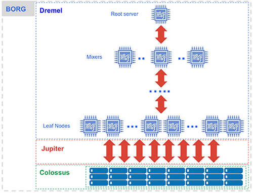
Google was among the first to bring this concept to the cloud with BigQuery (finally!) together with AWS Redshift and Snowflake (image from Google Blog).
Under the hood, BigQuery comprises five different main components:
- Storage service Colossus (and columnar format Capacitor).
- Compute service Dremel.
- Network service Jupiter.
- Orchestration service Borg.
This architecture is also common among the cloud data warehouse3, offering users tremendous query power in exchange for cash.
For storage and compute service, you can see one of my blog post where I used S3 and Spark to illustrate storage and processing at scale: https://hung.bearblog.dev/recsysoff/.
Using BigQuery
Cloud data warehouse can help you make sense of TBs of your data, but it can also burn all the cash in your wallet. There are horror stories and complaints, and it's up to you to remember to do your homework.
First, BigQuery billing system. Compute and storage are separated, and they are also billed separately. Storage is simple, you pay for the amount of data you store past a free limit. This is the same for all cloud data warehouse.

For compute, BigQuery charges per GB processed, which means $6.25 per TB on-demand or prepaid cost called "capacity" that should be cheaper for contracted customers4. This pricing model creates quirky behavior, such as
"When you run a query, you're charged according to the data processed in the columns you select, even if you set an explicit
LIMITon the results."
For this, BigQuery users are expected to safeguard themselves and use features such as partitioning and clustering.

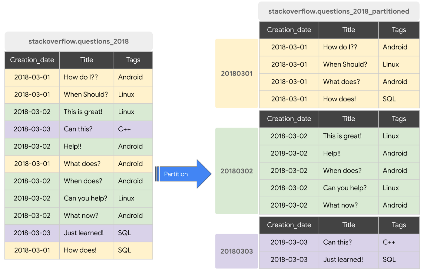
Partitioning in BigQuery means dividing your logical table into slices based on a range, typically a datetime range e.g., ingestion date or an INTEGER column. This helps to reduce the size of data scanned in applicable queries with WHERE clause (image from Google's blog post).

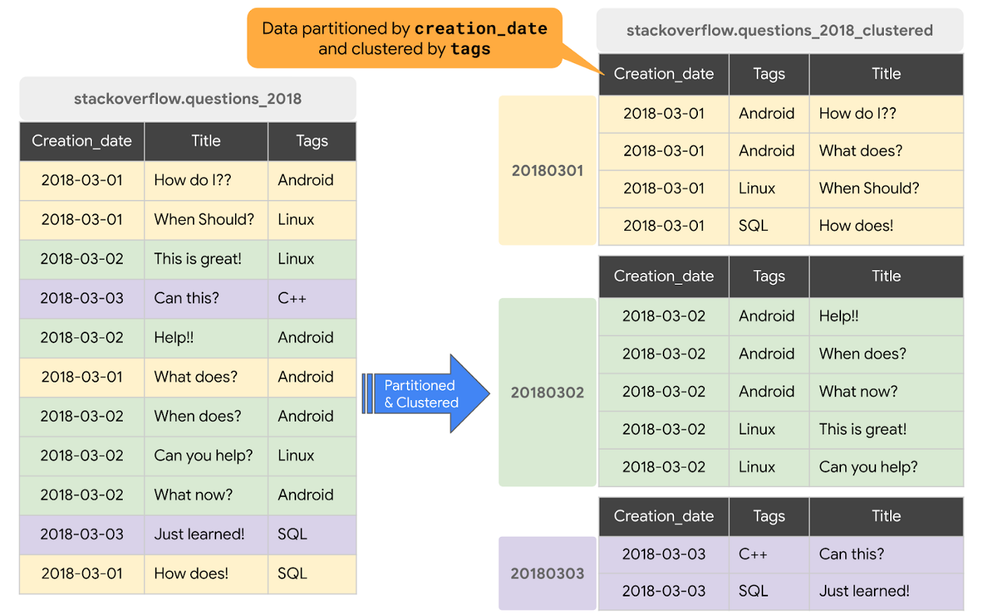
If partitioning is like filtering in advance, then clustering is sorting in advance. The operation ensures that records sorted by the same value in a column(s) are colocated. This can further reduce data scanned and increase speed for filtering and aggregation queries.
Let's see these in actions with the homework.
Other tidbits
- Avoid
SELECT *. - Use/Read BigQuery price estimator before actually running.
- Materialize queries in stages i.e., explicitly create temporary table for intermediate results for complex queries.
- On a similar note, instead of join then filter like in a normal SQL database, filter the data aggressively (to temporary tables) before joining them.
- Arrange join tables in decreasing order of size in queries.
- CTE
WITHexpression in BigQuery is not a "repared statement", meaning the CTE result is not cached but always re-evaluated. This can blow up your cost in query referencing the CTE multiple times. Use temporary table instead.
Homework
The table used is NYC Yellow Taxi Data for the first 6 months of 2024, imported into BigQuery first as an external table from GCS (ny_taxi.yellow_tripdata) and then as a native table (ny_taxi.mv_yellow_tripdata).


I created the external table from the UI, but it should be creatable with SQL
CREATE OR REPLACE EXTERNAL TABLE `ny_taxi.yellow_tripdata`
OPTIONS (
  format = 'PARQUET',
  uris = ['gs://kestra_archive_bucket/yellow_tripdata_2024-*.parquet']
);

--

CREATE OR REPLACE TABLE `solid-acrobat-440004-g5.ny_taxi.mv_yellow_tripdata` AS (
  SELECT *
  FROM `solid-acrobat-440004-g5.ny_taxi.yellow_tripdata`
);
Question 1
Besides running COUNT query, the number of rows can be viewed through the metadata tab for tables.

Question 2
Support for external table is limited in BigQuery. This also means the query estimator will show 0 bytes instead of the value in the materialized table.

Question 3
BigQuery stores data in columnar format, so the amount of data scanned depend on the number of columns asked in the query. That means querying 2 columns will lead to a higher estimate of bytes scanned than 1 column.
Question 4
Nothing to note
Question 5
The pattern "your query will always filter based on tpep_dropoff_datetime and order the results by VendorID" tells us that the table is best partitioned by tpep_dropoff_datetime and clustered by VendorID. The new table can be created with
CREATE OR REPLACE TABLE ny_taxi.yellow_tripdata_partitioned_clustered
PARTITION BY DATE(tpep_dropoff_datetime)
CLUSTER BY VendorID
AS
SELECT *
FROM ny_taxi.mv_yellow_tripdata;
Question 6
The difference between the partitioned and non-partitioned tables can be view in the cost estimator.
Question 7
External table data still resides in its original location - GCS bucket in this case.
Question 8
Clustering introduces overhead, which can harm performance instead e.g., for small tables.
Question 9
Lastly, COUNT query for materialized table in BigQuery incurs 0 bytes cost as metadata is cached.
Conclusion
And that's it for module 3. Next week, I will learn about dbt with Module 4: Analytics Engineering!
References
- Kleppmann, M. (2017). Designing Data-Intensive Applications : The Big Ideas behind Reliable, Scalable, and Maintainable Systems (First edition, second printing). O’Reilly Media.
- Ghemawat, S., Gobioff, H., & Leung, S. T. (2003, October). The Google file system. In Proceedings of the Nineteenth ACM Symposium on Operating Systems Principles (pp. 29-43).
- Dean, J., & Ghemawat, S. (2008). MapReduce: simplified data processing on large clusters. Communications of the ACM, 51(1), 107-113.
- Tereshko, T. and Tigani, J. (2016) BigQuery under the hood: Google’s Serverless Cloud Data Warehouse. Google. Available at: https://cloud.google.com/blog/products/bigquery/bigquery-under-the-hood (Accessed: 14 February 2025).
- Dean, H., & Denis, S. (2021). Colossus under the hood: A peek into Google’s scalable storage system. Accessed February, 14.
- Verma, A., Pedrosa, L., Korupolu, M., Oppenheimer, D., Tune, E., & Wilkes, J. (2015, April). Large-scale cluster management at Google with Borg. In Proceedings of the Tenth European Conference on Computer Systems (pp. 1-17).
- Melnik, S., Gubarev, A., Long, J. J., Romer, G., Shivakumar, S., Tolton, M., ... & Shute, J. (2020). Dremel: A decade of interactive SQL analysis at web scale. Proceedings of the VLDB Endowment, 13(12), 3461-3472.
- Singh, A., Ong, J., Agarwal, A., Anderson, G., Armistead, A., Bannon, R., ... & Vahdat, A. (2015). Jupiter Rising: A Decade of Clos Topologies and Centralized Control in Google's Datacenter Network. ACM SIGCOMM Computer Communication Review, 45(4), 183-197.
- Thallam, R. (2020) BigQuery explained: Storage overview, and how to partition and cluster your data for optimal performance. Google. Available at: https://cloud.google.com/blog/topics/developers-practitioners/bigquery-explained-storage-overview (Accessed: 14 February 2025).
Often referred as "disaggregation of storage and compute".↩
SQL interface also becomes the standard for big data processing framework, with the release of Spark SQL for Spark 3.0, Trino (formerly Presto), together with the cloud data warehouse. SQL is not just a language, it's now a protocol.↩
BigQuery is the original data lakehouse. Databricks just market the term. On the other hand, Google seems to have a history of having everything in hand then fumble at the race (definitely not talked about Transformer and LLM situation). But well, a bad start may mean nothing in a marathon.↩
The compute cost is what varies between cloud data warehous e.g., Snowflake charges per second of query execution instead.↩
