Build a Search Engine
What's this?
This is a tutorial to build a minimal text search engine (afterwards only referred to as search engine) in Python, based on the workshop to prep for the LLM Zoomcamp course from DataTalks.Club. The workshop centered around the problem of building a text search engine.
Suppose we have a corpus i.e., a collection of documents, each containing text content of arbitrary length. We have a question, or a query, and we want to search for the answer in the content of the document. Effectively search and return the most relevant document to the query, or the closest answer to the question, is the goal of information retrieval, a hot field of research right now. The central idea in the field right now is vector search. Take a look at closest answer. How do we measure the distance between a document and a query? Well, if we can turn them into vectors, then we can use vector distance as proxy - the most relevant document will be the one whose vector representation is closest to the query's vector representation.
The workshop advanced through ways to create these vector representations (or more formally, embeddings), from literal embeddings e.g., bag or words to semantic representations e.g., BERT output.
Setup
The workshop repo: https://github.com/alexeygrigorev/build-your-own-search-engine.
The Python environment requires these libraries:
pip install requests pandas scikit-learn jupyter
The dataset used for the workshop is the JSON-ified version of the courses' FAQs: https://github.com/alexeygrigorev/llm-rag-workshop/raw/main/notebooks/documents.json.
The dataset can be downloaded and stored in a Python list of dictionaries with the code snippet.
import requests

docs_url = 'https://github.com/alexeygrigorev/llm-rag-workshop/raw/main/notebooks/documents.json'
docs_response = requests.get(docs_url)
documents_raw = docs_response.json()

documents = []

for course in documents_raw:
    course_name = course['course']

    for doc in course['documents']:
        doc['course'] = course_name
        documents.append(doc)
Each element in documents will have 4 keys: course, section, question, and text, which is the answer to the question.
For easier processing, documents will be turned into a pandas DataFrame.
import pandas as pd

df = pd.DataFrame(documents, columns=['course', 'section', 'question', 'text'])
The problem for the workshop is retrieving relevant FAQs based on a user's query. Formally, this is an information retrieval problem, one with an interesting history of development. In the workshop, we will go from literal search with techniques based purely on the word letters (e.g., bag of words) to semantic search, where the word's meaning is used in searching.
Literal search
Bag of words
This is a basic way to represent the documents. In bag of words model, a document is reduced to the equivalent of a Python dictionary of word frequency. Order (and grammar) is discarded. For example, the English sentence "I am a cat" will be reduced to {"I": 1, "am": 1, "a": 1, "cat": 1}.
In scikit-learn, this is implemented via CountVectorizer. Its effect on some examples below.
from sklearn.feature_extraction.text import CountVectorizer

docs_example = [
    "January course details, register now",
    "Course prerequisites listed in January catalog",
    "Submit January course homework by end of month",
    "Register for January course, no prerequisites",
    "January course setup: Python and Google Cloud"
]
# stop_words tells the instance to not count common
# but unmeaningful words such as "a" or "the".
cv = CountVectorizer(stop_words='english')
X = cv.fit_transform(docs_example)

names = cv.get_feature_names_out()
df_docs = pd.DataFrame(X.toarray(), columns=names).T
Different from a true word frequency count, the fit method of CountVectorizer limits the words to count frequency to only those appearing in the training data.
So for the example "I am a cat" above, the current cv will output an empty count since none of the words appear in its defined vocabulary names of
array(['and', 'by', 'catalog', 'cloud', 'course', 'details', 'end', 'for', 'google', 'homework', 'in', 'january', 'listed', 'month', 'no', 'now', 'of', 'prerequisites', 'python', 'register', 'setup', 'submit'], dtype=object)
For df_docs, it will be a matrix of each word frequency for each document (each string denoted by position in the Python list in this case) that looks like below.
| 0 | 1 | 2 | 3 | 4 | |
|---|---|---|---|---|---|
| catalog | 0 | 1 | 0 | 0 | 0 |
| cloud | 0 | 0 | 0 | 0 | 1 |
| ... |
TF-IDF
Term frequency–inverse document frequency or TF-IDF is a way to measure the importance of a word in each document in a corpus.
It is the product of 2 terms: term frequency and inverse document frequency. The exact formulae for TF-IDF and related terms can be found here. Intuitively, the importance of a word in a document is proportional to how many times it appears in that document but offset by the number of documents it appears in1.
In scikit-learn, it is implemented via TfidfVectorizer
from sklearn.feature_extraction.text import TfidfVectorizer

cv = TfidfVectorizer(stop_words='english')
X = cv.fit_transform(docs_example)
df_docs = pd.DataFrame(X.toarray(), columns=names).T
df_docs.round(2)
The result will be a table with column and row names similar to one from CountVectorizer, but the values are score instead of frequency.
| 0 | 1 | 2 | 3 | 4 | |
|---|---|---|---|---|---|
| catalog | 0 | 0.57 | 0 | 0 | 0 |
| cloud | 0 | 0 | 0 | 0 | 0.47 |
| ... |
Search
We need to vectorize the query the same way i.e., count the frequency or calculate TF-IDF for the same vocabulary of words before we can calculate the distance and determine the most relevant documents.
query = "Do I need to know python to sign up for the January course?"
q = cv.transform([query])
query_dict = dict(zip(names, q.toarray()[0]))
query_dict
This would yield the dictionary. Only words that are in the vocabulary of TfidfVectorizer cv (built from from the documents) were counted.
{'catalog': 0.0,
 'cloud': 0.0,
 'course': 0.39515588491314224,
 'details': 0.0,
 'end': 0.0,
 'google': 0.0,
 'homework': 0.0,
 'january': 0.39515588491314224,
 'listed': 0.0,
 'month': 0.0,
 'prerequisites': 0.0,
 'python': 0.8292789960182417,
 'register': 0.0,
 'setup': 0.0,
 'submit': 0.0}
There are many way to find the similarity between 2 vectors. The simplest that works is cosine similarity, or the inner product between 2 vectors divided by product of the lengths. In sci-kit learn it would be
from sklearn.metrics.pairwise import cosine_similarity
cosine_similarity(X, q)
which yields
array([[0.25955955],
       [0.21371415],
       [0.17843726],
       [0.28419115],
       [0.57137158]])
A faster way is just
X.dot(q.T).toarray()since TF-IDF is already a normalized vector i.e., has length 1.
We can now do it for all documents.
fields = ['section', 'question', 'text']
transformers = {}
matrices = {}

for field in fields:
	# min_df species the frequency cut-off that a word must have
    cv = TfidfVectorizer(stop_words='english', min_df=3)
    X = cv.fit_transform(df[field])

    transformers[field] = cv
    matrices[field] = X
transformers store the 3 vectorizers for the 3 fields. Their names can be extracted with transformers['text'].get_feature_names_out(). matrices contains the TF-IDF for each field. Now we can calculate similarity between a query and the field(s) of all documents.
query = "I just singned up. Is it too late to join the course?"

q = transformers['text'].transform([query])
score = cosine_similarity(matrices['text'], q).flatten()
We can sort the answer based on this score.
import numpy as np
idx = np.argsort(-score)[:10]
score[idx]
df.iloc[idx].text
Additionally, we can filter for another field
mask = (df.course == 'data-engineering-zoomcamp').values
score = score * mask
Putting everything up to now together.
import numpy as np
query = "I just singned up. Is it too late to join the course?"

q = transformers['text'].transform([query])
score = cosine_similarity(matrices['text'], q).flatten()
mask = (df.course == 'data-engineering-zoomcamp').values
score = score * mask
idx = np.argsort(-score)[:10]
df.iloc[idx].text
Boosting & Filtering
Up until now, we assume that each field in a document holds the same importance in searching. But there can be some field that we deem more importance. Boosting is the act of increasing the contribution of some field to the score in search. It's simply multiplying the score of the field by a constant in calculation of the total.
boost = {'question': 3.0}

score = np.zeros(len(df))

for f in fields:
    b = boost.get(f, 1.0)
    q = transformers[f].transform([query])
    s = cosine_similarity(matrices[f], q).flatten()
    score = score + b * s
Filtering is when we select or discard documents whose some field meet or do not meet some value. In linear algebra, this is done via multiplying the matrix element-wise with a boolean mask, whose value will be 1 (True) at element position that meets the condition and 0 (False) otherwise2.
filters = {
    'course': 'data-engineering-zoomcamp'
}

for field, value in filters.items():
    mask = (df[field] == value).values
    score = score * mask
Putting it all together: minsearch
The minimal functionalities were put together in a class that loosely resembles scikit-learn API that can be found at https://github.com/alexeygrigorev/minsearch/blob/main/minsearch.py.
Semantic search
Up until now we only care about exact matches of a word, only its literal letters. The performance can be enough, but we are not using the word meaning, something equally, if not more, important compared to its letters. A particular case will be heteronym - word that looks the same but have unrelated meaning based on context. For example, Google must treat the "address" in "address of nearest McDonald's" different from one in "how to address your annoying older relative". This is where modern semantic embeddings come in.
Literal embedding attempts to capture the whole document, with each word a dimension with a single score capturing its importance. And there are many 0s because not all words in the vocabulary will appear in the document.
Semantic embedding attempts to capture only a single word. Each word receives a dense vector of fixed dimensions. Each dimension representing an abstract aspect of its meaning3.
Matrix Factorization
Before using deep learning model, we can create dense vector by using matrix decomposition techniques on the bag or words or TF-IDF. By right, they are used for dimensionality reduction and other problems, but can be used here to create a dense vector representation for each word. Of course, since bag of words does not hold any information about word order so the embedding will not produce word order, but it may be able to capture synonyms.
Latent semantic analysis (LSA) implemented via sklearn.decomposition.TruncatedSVD is a particular decomposition technique applied on term-count/TF-IDF. Example of using it in scikit-learn.
from sklearn.decomposition import TruncatedSVD

X = matrices['text']
cv = transformers['text']

svd = TruncatedSVD(n_components=16)
X_emb = svd.fit_transform(X)

query = 'I just singned up. Is it too late to join the course?'

Q = cv.transform([query])
Q_emb = svd.transform(Q)
score = cosine_similarity(X_emb, Q_emb).flatten()
idx = np.argsort(-score)[:10]
list(df.loc[idx].text)
You can see that the result is not good - all 10 documents missed the correct one (at least for me).
LSA can produce vector with negative elements. If you want to avoid this due to these hard-to-interpret dimensions, you can use decomposition techniques that produce non-negative matrix such as (unsurprisingly) Non-Negative Matrix Factorization (NMF). Example of using it in scikit-learn.
from sklearn.decomposition import NMF

nmf = NMF(n_components=16)
X_emb = nmf.fit_transform(X)
Q = cv.transform([query])
Q_emb = nmf.transform(Q)
score = cosine_similarity(X_emb, Q_emb).flatten()
idx = np.argsort(-score)[:10]
list(df.loc[idx].text)
The result is slightly better since the correct document is found in the result (but it's still not up in the top).
BERT
State-of-the-art (SOTA) semantic embeddings are often produced from a deep learning model pretrained on a large corpus. Semantic embedding is produced with certain characteristics. For example, synonyms will have similar embeddings, while a heteronym will have a different embedding depending on the context. Another property is "distance" between similar pair of words, with the most famous example King - Man + Woman = Queen.
The current SOTA embeddings come from transformers, the most common one is BERT. The embedding will be the output of the last layer but before passing to the linear layer4.
The easiest way to use BERT is using Hugging Face's transformers library.
import torch
from transformers import BertModel, BertTokenizer

tokenizer = BertTokenizer.from_pretrained("bert-base-uncased")
model = BertModel.from_pretrained("bert-base-uncased")
# model = model.to("cuda") # if have GPU e.g., Colab
model.eval() # Set the model to not training.
To pass text through model, first we need to tokenize i.e., break the text into smaller chunks known as tokens. For that, we use a tokenizer that is built specifically for each transformer model. For Enlighs, this is for the most part similar to breaking down a sentence into words.
Afterwards, we pass the tokens through the model to get the embedding for each token. For BERT, each embedding will have 768 dimensions, but the model also outputs one embedding for each input token, so the shape of last_hidden_state is (2, 15, 768) in the workshop. We need to pool the embedding values by taking the max or mean to create the final embedding.
The full example of embedding the documents and searching in its is provided below.
from tqdm.auto import tqdm

def make_batches(seq, n):
    result = []
    for i in range(0, len(seq), n):
        batch = seq[i:i+n]
        result.append(batch)
    return result

def compute_embeddings(texts, batch_size=8):
    text_batches = make_batches(texts, 8)

    all_embeddings = []

    for batch in tqdm(text_batches):
        encoded_input = tokenizer(batch, padding=True, truncation=True, return_tensors='pt')
        # encoded_input = encoded_input.to("cuda")
        with torch.no_grad():
            outputs = model(**encoded_input)
            hidden_states = outputs.last_hidden_state

            batch_embeddings = hidden_states.mean(dim=1)
            batch_embeddings_np = batch_embeddings.cpu().numpy()
            all_embeddings.append(batch_embeddings_np)

    final_embeddings = np.vstack(all_embeddings)
    return final_embeddings

embeddings = {}
# fields = ['section', 'question', 'text']

for f in fields:
    print(f'computing embeddings for {f}...')
    embeddings[f] = compute_embeddings(df[f].tolist())

query = "I just singned up. Is it too late to join the course?"
encoded_input = tokenizer(query, padding=True, truncation=True, return_tensors='pt')
# encoded_input = encoded_input.to("cuda")
with torch.no_grad():
    outputs = model(**encoded_input)
    hidden_states = outputs.last_hidden_state
sentence_embeddings = hidden_states.mean(dim=1)
sentence_embeddings = sentence_embeddings.cpu().numpy()

boost = {'question': 3.0}
score = np.zeros(len(df))

for f in fields:
    b = boost.get(f, 1.0)
    s = cosine_similarity(embeddings[f], sentence_embeddings).flatten()
    score = score + b * s

filters = {
    'course': 'data-engineering-zoomcamp'
}

for field, value in filters.items():
    mask = (df[field] == value).values
    score = score * mask

idx = np.argsort(-score)[:10]
list(df.loc[idx].text)
Conclusion
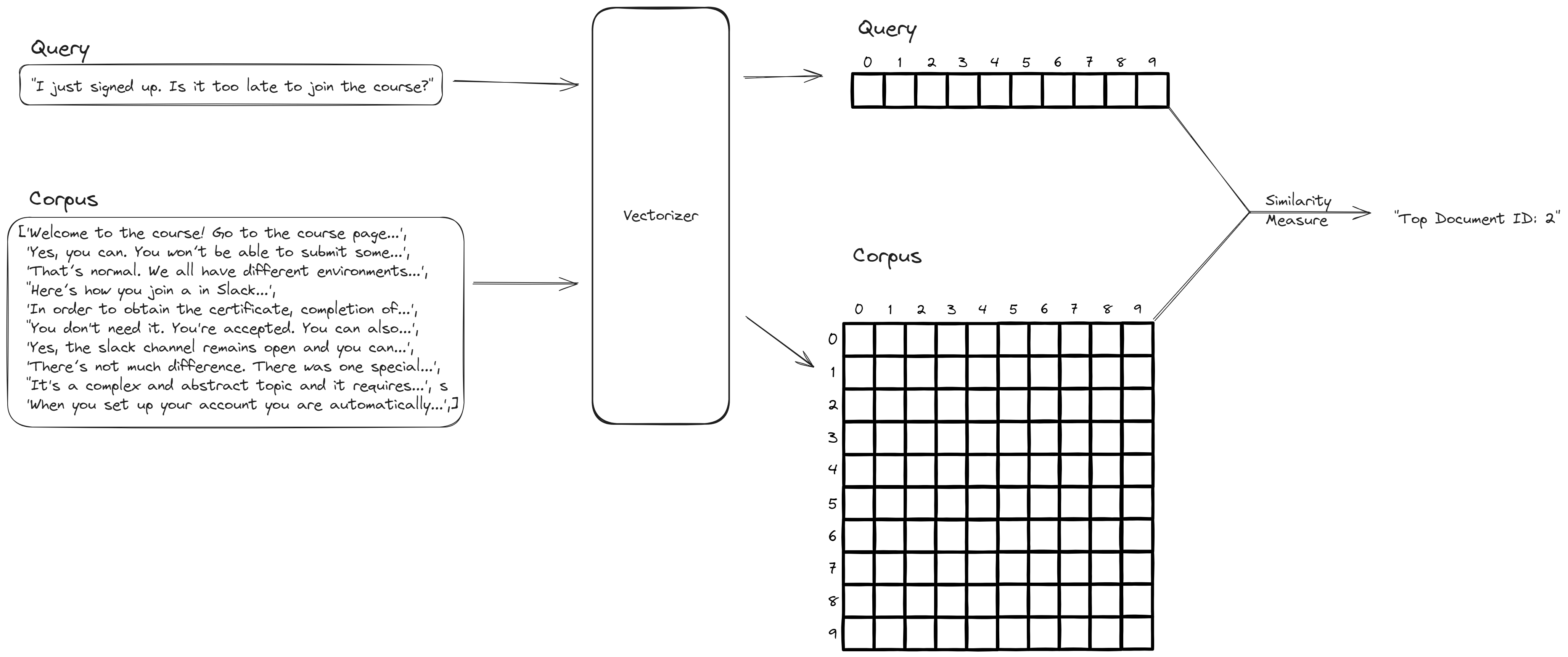
The workshop is structured around the problem of building a search engine for finding relevant documents from a corpus based on a query. The solution to it is in the figure below, with the key step being transforming the text in corpus and query into vectors then use vector distance(s) to determine which documents are relevant.
 I hope my notes have been helpful, and you have fun while learning from the LLM Zoomcamp.
It could be practically thought of as a normalized version of bag of words count.↩
NumPy refers to this as boolean indexing.↩
A collection is now a collection of vectors, or matrix instead of being just a vector. The sheer bigger size represents more information captured for each document.↩
This is similar to how in computer vision people use the output of the last layer of model such as ResNet as embedding for the image.↩